⭕️ 3D Positioning with only Two Motors
Achieving 3-axes of microscopy imaging with just a motor and a linear actuator.
Athelas One is our signature device - an FDA Cleared 3-Minute blood diagnostics tool used by thousands of patients across North America. We pair cutting-edge hardware with CNN models to segment and analyze the cellular composition of one’s blood. Right now, we can quantify lymphocytes, neutrophils, hemoglobin, and platelets — the essential components of a traditional ‘complete blood count’ — at a fraction of the cost of most blood analyzers. This simplicity and affordability gives allows us to deploy blood analyzers in more places, including patients’ homes.
Athelas One was a complex endeavor and we faced many hurdles during its development. Here’s one of the many interesting problems we had to solve:
The Problem - Achieving 3 axes of microscopy motion
At its core, Athelas One is simple - the device pans a glass slide under a stationary microscopic camera and captures images from multiple regions. In such a sampling problem, the accuracy of your estimate can increase as you sample more data. Naturally we wanted to increase the number of regions we can image.
Initially, Athelas One was capable of moving a blood sample slide in two dimensions using two linear actuators in Y and Z. But we realized there would be a huge sampling improvement if we could move in the third dimension as well: the X axis.
The Constraints - Keeping just 2 motors
The most obvious solution to this would be adding a 3rd motor to drive the slide in X. However, we found that the integration work would be a painful choice given our small form factor. It would require an electrical redesign of our device and take months to complete.
But then we had a thought - what if we could achieve 3 axes of motion with the existing 2 motors?
The solution - Parallelograms
We found that the key was to trace a parallelogram pathway that gave us an additional degree of freedom.
When we move the new stage left or right all the way, it runs into an angled rail that pushes the stage up or down. This isn’t true arbitrary 3D path motion, but it’s enough to give us the ability to move the camera view from any 3D point on the slide to any other 3D point, which is all we really need. It takes three steps instead of one, but our motor doesn’t mind the extra work.

We designed and manufactured these 3D-capable units in only a few months in late 2020, and we had units ready to go at the end of December. However, there was still one missing piece.
The Calibration - Using computer vision to determine the boundaries of the parallelogram
Moving to any position with this 3-step dance required knowledge of the exact dimensions of the accessible parallelogram. Namely, we wanted to know what linear actuator position brought us to a given corner. And we didn’t trust the manufacturing tolerances nor the linear actuator encoders to be consistent enough. Calibration is a necessity when building hardware products with many moving pieces.
Since our device has a camera and CPU onboard, we developed a way for the camera to visually detect if it had reached a corner. This allows it to calibrate itself in our factory without any operator effort.
All it has to do is:
Drive the stage as far forward as it can go. Record this linear actuator position as Corner A.
Drive the stage backwards. Use the camera to detect when the direction of travel changes, and record that position as Corner C.
Continue driving the stage backwards as far as it can go, and record that position as Corner D.
Drive the stage forwards again until the direction of travel changes, and record that position as Corner B.
With a bit of effort and a few late nights, we got this calibration algorithm up and running, and we are just about to start shipping our customers a 3rd dimension for the price of two motors.
It may seem like we glossed over the hardest part of this process - which we did: how exactly did we use the camera to tell when the stage turns a corner?
The solution involved designing a special calibration slide with a visual color-code so that when the stage moves up or down, the camera would be able to tell.
Designing the color-coded slide for computer vision
In essence, calibration starts with a simple step: comparing a known with an unknown to figure out the difference in value. We needed to build our own “known” - a reliable constant all of our devices could be calibrated based on. Our constant took the form of a colored test strip.
Step 1: X-encoding
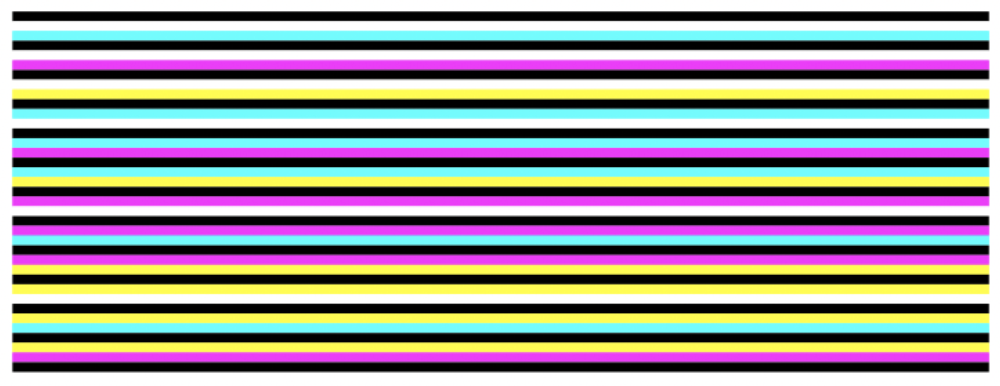
First, we had to encode horizontal distance onto a slide that was detectable even by a camera with a tiny field of view. We did so by creating the color bar code below. Each non-black color in the code represents a number:
These colors and our barcode image may seem random, but everything was chosen for a specific reason. First, these five are the colors most standard office printers are best at producing - white, cyan, magenta, yellow, and black.
Second, we chose the width of the stripes by iterating to find the smallest width our printer could produce repeatably. (We could have outsourced some ultra-high quality prints, but here at Athelas our culture is all about moving quickly and delivering good engineering the same day with what you have on hand whenever possible).
Third, this is the key for our code itself:
White: 0Cyan: 1Magenta: 2Yellow: 3Black: delimiter
Reading from top to bottom in the image, you can see our pattern is:
_01_02_03_10_12_13_20_21_23_30_31_32_These are nice, distinct, increasing numbers (we omitted double color stripes like 11 just to be safe). So now when our camera takes a tiny picture somewhere on this pattern, we have a way for it to determine the X-position of that picture on the slide.
You can try this for yourself: zoom in on the image until you can just see two colors between black bars. Then decode the colors into numbers, and you’ll know where you are.
With that, we have a workable code for horizontal distance! Using a regular ole’ office printer!
Step 2: Color recognition
Once we captured an image of a region, we needed to interpret the colors in the image to determine what X-position we were at. Here’s an example image and the associated X-position:

To interpret the image, we need to do the following steps:
Find the position of the black lines
Find the colors of the two regions adjacent to the left-most black line.
Finding the Black Line
Finding the black line was a simple use of HSV color masking. Here were the steps to do it:
Acquire an image with our camera.
Apply a Gaussian Blur to smooth the image.
Convert the image to HSV.
Apply an HSV color mask for the black region. This leaves us with only two colors: black and white.
Iterate over the image in X until we find a position where most of the pixels are black. Call that position the start of a black region. Keep going until the pixels turn white again. Call that the end of a black region.
Now that we found the black lines, we next needed to determine the colors of the regions adjacent to the black lines.
Step 3: Finding the colors of the regions
Finding the colors of adjacent regions followed a similar procedure of HSV masking. However, this was much trickier as we needed to carefully choose the correct ranges for the HSV color masks. We did so by creating 3d HSV plots of strips of color in our images so that we could visually get a quick sense of the HSV boundaries:

This allowed us to get a rough sense of what the expected ranges should be. Once we had the ranges, we carried out the following steps:
Apply each of 4 color masks on the image (white, cyan, yellow, magenta).
Select the mask with the most pixels as the color of the strip.

We then mapped the colors to an x-distance, using our barcode rules:
Color-Pair            X-Distance
--------------------------------
yellow-cyan           1
yellow-magenta        2
yellow-white          3
...
...
OK! Now that we had an X-position corresponding to number of linear actuator steps, we could begin determining corners.
Step 4: Getting corner position from the data
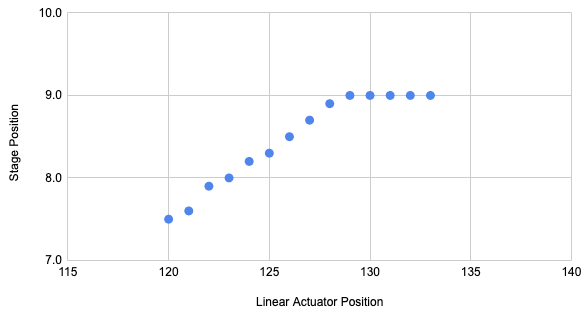
When we move the stage back one step at a time and record the X-position, we get data like this:
To a human, finding the corner in this dataset is easy. But how could we do this algorithmically? Fortunately, a friend of ours had solved a similar problem a while ago and suggested a great method:
For each index in the X-ordered data set, split the data set at the current index into two sets.
Fit two linear regressions to the points before and after the index, and calculate the total absolute residual error of that model.
The index that leads to the lowest absolute error is at the corner.
Once you do that for each corner in a real data set, here’s what it looks like!

That’s a pretty parallelogram! So our device is now able to find the exact linear actuator positions that correspond to each corner in our stage without any human help.
Summary
At Athelas, we leverage software and computer vision to allow our hardware teams to move fast - that’s one of our biggest advantages as a company. This was a great example of how we were able to use software to get away with imperfect tolerances in our hardware. We didn’t need to add a third motor if we could make it happen with clever software. And we didn’t need our parallelogram corners to be perfectly repeatable as we could write a calibration program to detect corners for every unit we make. As a result our costs were lower, our manufacturing speeds were faster, and we were able to ship a production-ready device in a fraction of the time.
We apply this principle throughout our product line, and this is just one example of how we believe a modern hardware company should work - a tight synthesis of hardware and software that allows the company to operate at much faster speeds than before.
If you’re interested in working on fascinating problems like this at the intersection of hardware, software, and healthcare, come join us! We’d love to hear from you at careers@athelas.com, or apply at our job board below:


